Topic inference visualization

In this page we will be visualizing the inference of topics in an image dataset and a text dataset. We will be using, as in most examples, the console applications which are readily available once you install LDA++. The image dataset is the well known Olivetti Faces and the textual dataset is the 20 news groups. Besides LDA++ will use scikit-learn to fetch the datasets and matplotlib and wordcloud to plot the inference process. All those libraries are very easily installed using pip or you could download anaconda for a full python distribution.

Fetching the datasets

We will use scikit-learn to fetch and preprocess the datasets in a few lines of python. The purpose of this example is to visualize the inference process and not to produce the best possible topics so shortcuts will be taken to save computation and experimentation time.

For simplicity you can download the following code as a script.

In [1]: import numpy as np
In [2]: from sklearn.datasets import fetch_olivetti_faces, fetch_20newsgroups
In [3]: faces = fetch_olivetti_faces()
In [4]: with open("/path/to/faces.npy", "wb") as f:
   ...:     np.save(f, (faces.data*255).astype(np.int32).T) # the pixels are normalized to [0, 1]
   ...:     np.save(f, faces.target.astype(np.int32))
   ...: 
In [5]: newsgroups = fetch_20newsgroups(
   ...:     subset="train",
   ...:     remove=("headers", "footers", "quotes")
   ...: )
In [6]: from sklearn.feature_extraction.text import CountVectorizer
In [7]: tf_vectorizer = CountVectorizer(max_df=0.9, min_df=2, max_features=1000,
   ...:                                 stop_words="english")
In [8]: newsdata = tf_vectorizer.fit_transform(newsgroups.data)
In [8]: with open("/path/to/news.npy", "wb") as f:
   ...:     np.save(f, newsdata.astype(np.int32).T)
   ...:     np.save(f, newsgroups.target.astype(np.int32))
In [9]: # Save the feature names in order to visualize the textual topics
In [10]: feature_names = tf_vectorizer.get_feature_names()
In [11]: import pickle
In [12]: pickle.dump(feature_names, open("/path/to/fnames.pickle", "w"))

Training LDA

After downloading the data and transforming them into the format readable by the console applications we can very easily infer topics from these datasets. We will use the --snapshot_every option to save a model from each epoch so that we can later visualize the inference process.

The following code trains two lda models one for the faces dataset and one for the 20 news groups. We infer 10 topics for the faces dataset and 20 for the text dataset. One should change the --workers option depending on the number of parallel threads his processor can execute.

$ lda train --topics 10 --iterations 100 \
>           --e_step_iterations 100 --e_step_tolerance 0.1 \
>           --snapshot_every 1 --workers 4 \
>           faces.npy faces_model.npy
E-M Iteration 1
100
200
...
$ lda train --topics 20 --iterations 100 \
>           --e_step_iterations 100 --e_step_tolerance 0.1 \
>           --snapshot_every 1 --workers 4 \
>           news.npy news_model.npy
E-M Iteration 1
100
200
...

After executing the above code (and the code from the previous section) the directory should contain the following files:

• faces_model.npy
• faces_model.npy_001 - faces_model.npy_100
• news_model.npy
• news_model.npy_001 - news_model.npy_100
• faces.npy
• news.npy
• fnames.pickle

As it is obvious the files (faces | news)_model.npy_(001 - 100) are the models for the corresponding epochs and we will be able to use them to plot the topic evolution.

Topic visualization

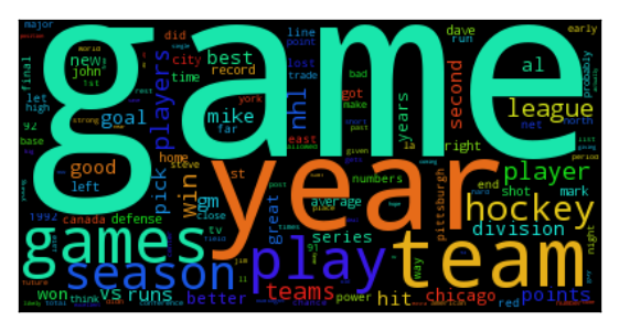
In order to visualize the evolution of the topics, firstly we need to visualize a topic. The faces dataset has been reformatted so that the topics can be visualized as a $64 \times 64$ image and the text topics will be represented by a wordcloud that emphasizes the most probable words.

The above images can be generated with the following code.

In [1]: import matplotlib.pyplot as plt
In [2]: import wordcloud
In [3]: import pickle
In [4]: import numpy as np
In [5]: def load_topics(path):
   ...:     with open(path) as f:
   ...:         _ = np.load(f)
   ...:         return np.load(f)
   ...: 
In [6]: # Visualize the faces topic
In [7]: f = plt.figure(figsize=(3, 3))
In [8]: plt.imshow(load_topics("faces_model.npy")[6].reshape(64, 64), cmap="gray")
Out[8]: <matplotlib.image.AxesImage at 0x7f41f8b7bf90>
In [9]: plt.xticks([])
Out[9]: ([], <a list of 0 Text xticklabel objects>)
In [10]: plt.yticks([])
Out[10]: ([], <a list of 0 Text yticklabel objects>)
In [11]: plt.tight_layout()
In [12]: f.savefig("path/to/image.png")
In [13]: 
In [13]: # Visualize the 20 newsgroups topic
In [14]: f = plt.figure(figsize=(4, 3))
In [15]: plt.imshow(
    ...:     wordcloud.WordCloud().fit_words(
    ...:         zip(
    ...:             pickle.load(open("fnames.pickle")),
    ...:             load_topics("news_model.npy")[0]
    ...:         )
    ...:     ).to_image()
    ...: )
Out[15]: <matplotlib.image.AxesImage at 0x7f41fcea6750>
In [16]: plt.xticks([])
Out[16]: ([], <a list of 0 Text xticklabel objects>)
In [17]: plt.yticks([])
Out[17]: ([], <a list of 0 Text yticklabel objects>)
In [18]: plt.tight_layout()
In [18]: f.savefig("path/to/image.png")

Topic evolution

In the following figure we have applied the above visualization for all the topics of the faces dataset for different epochs.

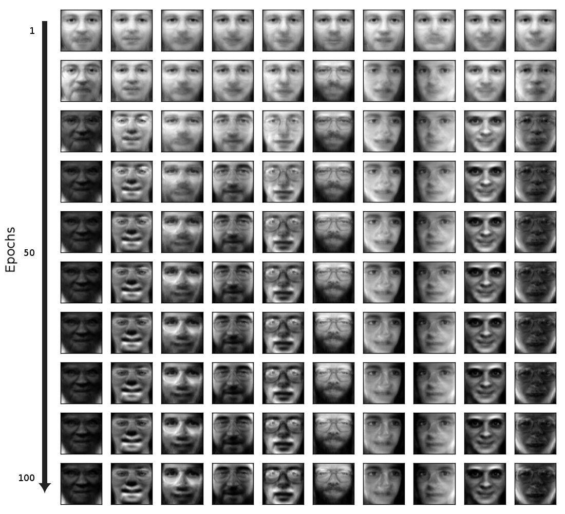
We can see that after one epoch all topics start from approximately the same position and it is really hard to predict what the final outcome will be for each topic. We can see clearly that there are topics that focus on some facial characteristics and not others. For instance, the second topic generates no mouths (hence the large black blob where the mouth would be) and the 6th topic generates beards.

We can perform the same visualization for the 20 news groups dataset but since the images of the wordclouds are larger we will visualize the inference of a single topic. We observe that the topics now converge much faster in the first tens of epochs.

Another attribute of a topic that we can visualize is the distribution over the words and its evolution. When the distribution over the words stops changing then the topic model has converged. It is common to check convergence using the likelihood instead. In the following figure we see the change in the distribution of the same topic as in the above figure. We see that indeed the topic changes very little from the 30th epoch and onwards.