MNIST dataset

The following example aims to point out the differences between the inferred topics of LDA and fsLDA. We decided to use the MNIST database which is a dataset of 70000 handwritten digits, in order to make the topics visualization more fancy!!! Both models are trained using the console applications that are thoroughly explained in the corresponding documentation page.

The console applications that are used in this example expect and save data in numpy format. We have already transformed the MNIST dataset to numpy format and you can download it if you copy and paste the following instructions in a terminal.

$ cd /tmp
$ wget "http://ldaplusplus.com/files/mnist.tar.gz"
$ tar -zxf mnist.tar.gz

Inspect MNIST dataset

We untar the mnist.tar.gz and load the extracted file, which corresponds to the training data, into a python session to inspect them.

In [1]: import numpy as np

# We load the training set
In [2]: with open("mnist_train.npy", "rb") as f:
   ...:     X_train = np.load(f)
   ...:     y_train = np.load(f)

# Print the shapes of X_train and y_train 
In [3]: X_train.shape
Out[3]: (784, 60000)

In [4]: y_train.shape
Out[4]: (60000,)

We observe that the training set is an array of size (784, 60000). All images in this dataset are $28\times28$ images, thus the first dimension is 784 (28*28=784), while the second dimension refers to the number of the training samples, which is 60000.

In the subsequent python session, we use the matplotlib library and the seaborn visualization library to plot 20 randomly selected training image. Both these libraries can be easily installed using pip.

In [5]: import matplotlib.pyplot as plt

In [6]: import seaborn as sns

# Set the aesthetic style of the plots
In [7]: sns.set_style("dark")

# Create 20 subplots
In [8]: fig, axes = plt.subplots(2, 10, figsize=(10, 2))

In [9]: for i in xrange(2):
   ...:     for j in xrange(10):
   ...:         axes[i][j].imshow(X_train[:, np.random.randint(0, 6000)].reshape(28, 28), cmap='gray_r', interpolation='nearest')
   ...:         axes[i][j].set_xticks([])
   ...:         axes[i][j].set_yticks([])

One possible output could be the following image.

Both in LDA and fsLDA, each document can be viewed as a mixture of various topics. However, the MNIST database consists exclusively of images, thus there is no direct analogy between words and documents. In order to use the MNIST dataset in combination with LDA and fsLDA we consider each image to be a document and each pixel in the image to be a word. As a result, our corpus consists of 70000 documents and the vocabulary size is 784.

Unsupervised LDA

In this section, we will visualize the inferred topics from an unsupervised LDA model using the lda application. We train an unsupervised model with 10 topics for 20 Expectation-Maximization steps, by setting the --topics argument to 10 and the --iterations argument to 20.

In addition, we initialize the topics as random distributions by using the --initialize_random option and use the --snapshot_every option to save a model after every epoch so that we can later inspect the topics evolution

$ lda train --topics 10 --iterations 20 \
>           --e_step_iterations 10 --initialize_random \
>           --random_state 25 \
>           --snapshot_every 1 --workers 4 \
>           mnist_train.npy mnist_lda_model.npy 
E-M Iteration 1
100
200
300
400
...
59900
60000
E-M Iteration 20
100
200
...
60000

After executing the above code the current directory should the following files:

• mnist_lda_model.npy
• mnist_lda_model.npy_001 - mnist_lda_model.npy_020

The first file is the final trained model, namely from the $20^{th}$ epoch, while the rest of the files are the trained models from the corresponding epochs and will be used to plot the evolution of the inferred topics during the epochs.

As we have already mentioned in previous documentation pages, the lda application trains a model and saves it as two numpy arrays. The first array is $\alpha$, namely the parameter of the Dirichlet prior on the per-document topic distributions, while the second one is $\beta$, which is the per-topic word distribution. Subsequently, in order to visualize the topics we merely have to visualize the $\beta$ parameter. In the following python session, we visualize the evolution of the inferred topics, during the training process.

In [1]: import numpy as np

In [2]: import matplotlib.pyplot as plt

In [3]: import seaborn as sns

In [4]: sns.set_style("dark")

In [5]: fig, axes = plt.subplots(10, 10, figsize=(10, 10))

In [6]: betas = []

In [7]: for i in xrange(1, 20, 2):
   ...:     with open("mnist_lda_model.npy_%03d" % i, "rb") as f:
   ...:         alpha = np.load(f)
   ...:         beta = np.load(f)
   ...:     betas.append(beta)
   ...: for e in xrange(10):
   ...:     for t in xrange(10):
   ...:         axes[e][t].imshow(betas[e][t, :].reshape(28, 28), cmap='gray_r', interpolation='nearest')
   ...:         axes[e][t].set_xticks([])
   ...:         axes[e][t].set_yticks([])

The following image depicts the evolution of 10 topics during the first 20 epochs. We observe that during the first epochs, it is rather hard to recognize any topic, however after the first 10 epochs, they seem quite converged.

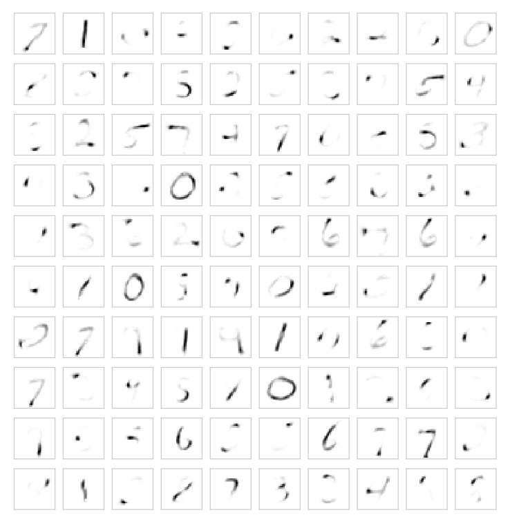
Subsequently, we train a new model with 100 topics, in order to observe the difference when the number of topics increases. The rest of the arguments remain the same as in the above example. The inferred topics are depicted in the following figure. If we observe the image from an overall perspective it is easily noticeable that some of the topics resemble numbers, while others seems to be part of numbers.

Fast Supervised LDA

In this section, we will visualize the inferred topics using the Fast Supervised LDA, using the fslda application. We retain the arguments from the previous section, so that we will be able to compare the inferred topics from the two variational inference methods. The following figure illustrates 100 topics, as they were inferred using Fast Supervised LDA.

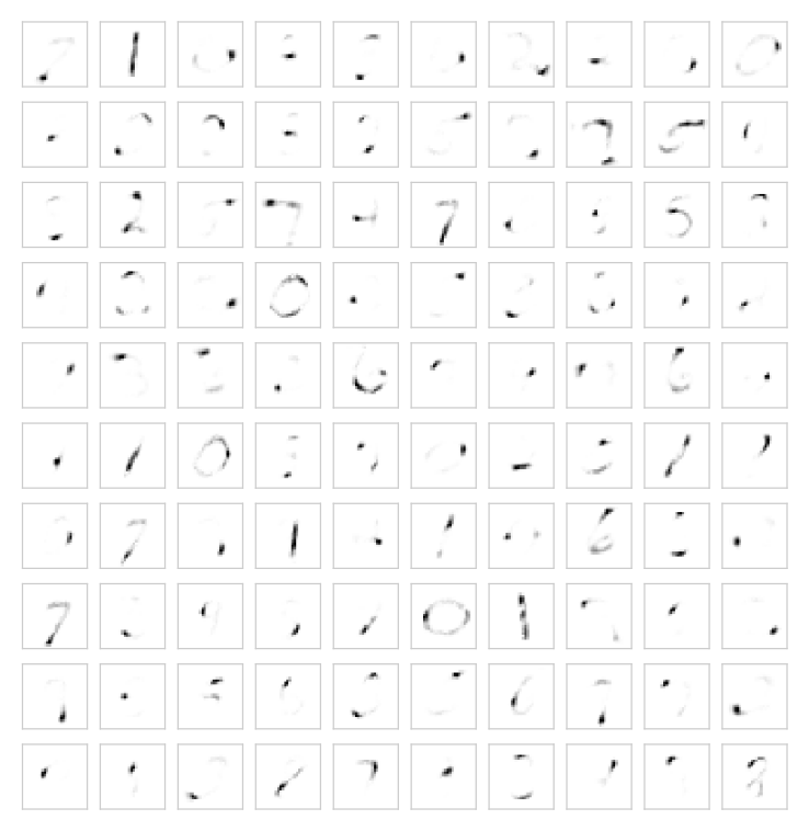
We observe that, the majority of the inferred topics using fsLDA is completely different with those using LDA. In addition, while in case of LDA many topics look like actual letters, in case of fsLDA the most of them looks like sections of letters.